Distributed Compressed Sparse Row

Introduction

About a year ago, I discovered Heat, a high performance tensor computation framework, in the Google Summer of Code 2022 website. At that time, I barely knew anything about distributed computing and message passing model of communication. I also had little understanding of how these huge scientific computing libraries worked under the hood. Despite my initial lack of knowledge, I decided to explore Heat and I’m very glad I did. In this blog, I talk about a project that I ended up working on for HeAT.

Helmholtz-Analytics Toolkit (HeAT)

Heat is a scientific computing library focussed on high performance data analytics in distributed cluster systems. It is built upon the PyTorch framework and uses torch.Tensors as its process local data structures. It allows huge amounts of data to be manipulated without being bound to the limitations of resources in a single system. But even then, there are use cases where the data is just so huge that holding it in memory is close to impossible. One such use case is in the field of neuroscience where large amounts of electrophysiology data is handled. The electrophysiology data is sparse in nature but even in its sparse representation, it requires memory distributed operations for practical computation due to its size. So, Heat needed a sparse module of its own. The first step towards creating a fully functioning sparse module is building a new sparse data structure, the Distributed Compressed Sparse Row Matrix (DCSR_matrix).

DCSR_matrix

Compressed Sparse Row is one of the most popular sparse representation formats. It was chosen as the first format to be supported by the heat.sparse module due to its simplicity and support in the PyTorch library. The CSR formats holds information only about the non-zero elements in the matrix. The DCSR_matrix splits the input object among the different process and deals with each chunk as an independent csr matrix. For most operations like elementwise addition, multiplication, etc…, the global information is unnecessary. And so, each process can operate independent of the others. This makes it very efficient to work with because there is not communication overhead.

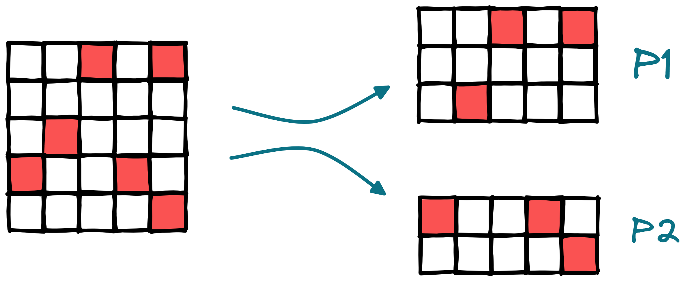
An example working with DCSR_matrix split along axis 0 across two processes.

Code:

import heat as ht
import torch

matrix = torch.as_tensor([[0, 0, 1, 0, 2],
                          [0, 0, 0, 0, 0],
                          [0, 3, 0, 0, 0],
                          [4, 0, 0, 5, 0],
                          [0, 0, 0, 0, 6]])

sparse_matrix = ht.sparse.sparse_csr_matrix(matrix, split=0) # DCSR_matrix

print(f"Sparse matrix: {sparse_matrix}")
print(f"Rank: {ht.MPI_WORLD.Get_rank()}, Local data: {sparse_matrix.larray}")
print(f"Local Data (in dense form): {sparse_matrix.larray.to_dense()}")

Output:

>>> mpirun -n 2 python3 example.py
Sparse matrix: (indptr: tensor([0, 2, 2, 3, 5, 6]), 
                indices: tensor([2, 4, 1, 0, 3, 4]), 
                data: tensor([1, 2, 3, 4, 5, 6]), 
                dtype=ht.int64, device=cpu:0, split=0)

Rank: 0, Local data: tensor(crow_indices=tensor([0, 2, 2, 3]),
                            col_indices=tensor([2, 4, 1]),
                            values=tensor([1, 2, 3]), 
                            size=(3, 5), nnz=3, layout=torch.sparse_csr)
Local Data (in dense form): tensor([[0, 0, 1, 0, 2],
                                    [0, 0, 0, 0, 0],
                                    [0, 3, 0, 0, 0]])

Rank: 1, Local data: tensor(crow_indices=tensor([0, 2, 3]),
                            col_indices=tensor([0, 3, 4]),
                            values=tensor([4, 5, 6]), 
                            size=(2, 5), nnz=3, layout=torch.sparse_csr)
Local Data (in dense form): tensor([[4, 0, 0, 5, 0],
                                    [0, 0, 0, 0, 6]])

Dense vs Sparse

Currently, the DCSR_matrix class supports the basic elementwise arithmetic operations but it is not fully usable in practical applications as important data manipulation operations such as matrix multiplication are not yet supported.

Let us compare the run times of a simple element-wise addition of two matrices done $10000$ times. This is the code I used to measure the performance of the two data formats.

import time
import heat as ht
import torch
import numpy as np

def generate_random_sparse(n = 100, threshold = 0.75, device=None):
    arr = torch.rand(n, n, device = device) # Generates uniformly distributed values from 0 to 1
    sparse_arr = torch.where(arr > threshold, 1., 0) # Applying this threshold gives us approximately threshold% of 1s in the matrix
    return sparse_arr

def func(t):
    start = time.perf_counter_ns()
    for _ in range(10000):
        _ = t+t
    end = time.perf_counter_ns()
    return end-start

device = ht.devices.gpu

sparsity = 0.999
size = 10000
for size in range(1000, 10001, 1000): # Use to observe effect of size
# for sparsity in (1 - np.logspace(-1, -5, num=5-1+1)): # Use to observe effect of sparsity
    torch_tensor = generate_random_sparse(size, sparsity, device.torch_device) # Generate random matrix of size nxn
    t = ht.array(torch_tensor, device=device) # Create a dense matrix (DNDarray)
    t_sparse = ht.sparse.sparse_csr_matrix(torch_tensor, device=device) # Create a sparse matrix (DCSR_matrix)

    print(f"{size},{sparsity},{func(t)},{func(t_sparse)}")

NOTE: This experiment might not really mimic any real life usecase but it should show the difference in efficiency between the two data formats.

The relative efficiency of sparse storage formats depends on the size and the sparsity of the array.

1. Size

The structure of sparse storage format entails a bit of extra computation that happens irrespective of the size of the matrix. This makes working with small matrices in sparse format relatively inefficient. But for matrices of large sizes, the extra bit of computation is very small in comparison. This is where sparse storage formats really shine.

The comparison is done between the dense array format (DNDarray) and the new sparse storage format (DCSR_matrix) for array sizes $(1000 \times 1000) \to (10000 \times 10000)$. The sparsity is fixed at $0.999$ for the experiment. The sparsity might seem extreme but it is not far from what is seen in most real life data like Netflix User x Movie watch data, Youtube Video Analytics, Amazon Customer data, Sensor input data from an IoT network, etc…

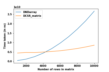
The graph clearly shows the differences in performance of the two formats. For matrix sizes less 4000, the extra computation makes DCSR_matrix less efficient but we can see the huge difference in computation when handling larger matrices.

NOTE: Real-life datasets are usually in the orders of $10^6$ - $10^9$ rows and columns. The limitation of memory on my laptop GPU did not allow me to test matrices larger than $10000$ rows. If you have a more powerful system at your disposal, definitely try out this experiment to really understand the performance gain.

2. Sparsity

Sparsity is the amount of “empty” space in the matrix.

$$Sparsity = \frac{Number\ of\ insignificant\ elements\ (Usually\ 0s)}{Total\ number\ of\ elements}$$

The sparse storage formats are more efficient with increased sparsity. To show this, in the next experiment, the size of the matrix is set at $(10000 \times 10000)$ and the sparsity is varied through the values $0.99, 0.999, 0.9999$ and $0.99999$.

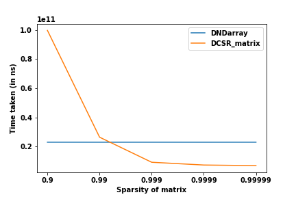
This shows that even at 90% sparsity, the dense format performs better. For the 99% sparsity, the two performances are almost the same (I suspect for larger matrices, this threshold will be even lower). As the sparsity increases, the time taken decreases exponentially for the sparse format while it stays the same for dense (as expected).

Scaling

In this project, we focused on two important aspects: sparseness of the matrix and distribution across processes. In the previous section, we explored sparsity, while in this section, we will try to see how well the data structure scales with increasing number of computational nodes. To test this, strong-scaling tests were conducted on the Jülich’s HDF-ML clusters (special thanks to Fabian!). In strong scaling, the workload is kept constant, and the number of compute nodes is increased to observe the effect.

For this experiment, the matrix size was kept fixed at $(25000 \times 25000)$. The runtimes of a dense matrix with those of sparse matrices of varying sparsity for a simple element-wise addition operation were recorded. The following graph shows the comparative runtimes between the two types of matrices.

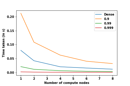
Even at 99% sparsity, the sparse version of the matrix beats the dense version by a huge margin.

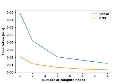
It can be seen from these graphs that the new sparse format scales in a similar manner to the dense format. This means sparse matrices can be used in distributed computing without incurring any handicap in terms of performance due to distribution.

Other miscellaneous aspects of development

SciPy style interface - SciPy has a very well established module that supports different types of sparse matrix formats. It is very popular among scientists who require easy-to-use libraries in their research. The only place where it falls short is the absence of support for parallel computation. When the size of data grows beyond a certain limit, SciPy becomes almost unusable. This is actually one of the core problems that HeAT aims to solve. In this module, the APIs are made to closely resemble the SciPy module APIs to ensure smooth migration of working code from SciPy to HeAT to run in high-performance computation clusters.
split = 0 - DCSR_matrix supports only splitting along the row-axis. It is a consequence of how the format is structured. It does not really make sense to distribute a Compressed Sparse Row Matrix along its column-axis.
todense() - The new module supports conversion of DCSR_matrix into a dense DNDarray. It will soon support the backward conversion too. This allows seamless transition between the two formats and improves developer experience.

Future of the project

Right now, the foundation of the class is complete. The addition of more element-wise operators like logical operations will be trivial. The implementation of matrix multiplication will be the next significant step. A Distributed Compressed Sparse Column class would make it easy to implement operations like matrix multiplication coupled with the DCSR_matrix class.

Conclusion

This project is the first step in building a fully-featured sparse module for HeAT. Furthur development of this project really has the potential to make a significant impact in the field of scientific computing. And I am really glad I could make a small contribution in that direction.

For me personally, this project was fun. I learnt a lot about distributed computing, unit testing and software design during the course of this project. I also really enjoyed working with the team at HeAT, especially Claudia. I look forward to seeing the future developments in the HeAT framework, especially, the sparse module.

Resources

HeAT - https://github.com/helmholtz-analytics/heat
Project PR - https://github.com/helmholtz-analytics/heat/pull/1028

Thank you for reading! Feel free to share your thoughts about this project in the comments. Also, don’t hesitate to get in touch with me.

Introduction#

Helmholtz-Analytics Toolkit (HeAT)#

DCSR_matrix#

Dense vs Sparse#

1. Size#

2. Sparsity#

Scaling#

Other miscellaneous aspects of development#

Future of the project#

Conclusion#

Resources#