Introduction
I have been meaning to learn the Reinforcement Learning with Verifiable Rewards (RLVR) training technique to finetune LLMs for a while now. During my internship at IBM, I had an opportunity to work on a project that involved fine-tuning language models with RLVR. It was the first time I finetuned LLMs and was a great learning experience. After my internship, I remained interested in gaining a deeper understanding of the algorithm. I wanted to see how far I can push the reasoning capabilities when training an LLM with this algorithm. I write this blog to document a set of experiments I ran on a toy task, along with the results and takeaways.
Github repo: https://github.com/Mystic-Slice/rl-grpo-countdown
Background
GRPO
Group Relative Policy Optimization is a reinforcement-learning algorithm used to training the latest reasoning models. It was first popularized by DeepSeek-R1. This algorithm removes the requirement for manual verification which is usually a huge bottleneck in training methods like RLHF or PPO. However, the scope of use for this algorithm is limited to tasks where responses can be verified programmatically (usually math, coding, MCQs, etc…). There are some ways to overcome this limitation (like using LLM-as-a-Judge to grade each response) but still not quite applicable to an arbitrary dataset.
I use the implementation of GRPO in the trl library which, more specifically, is the improved version of GRPO proposed by the DAPO paper.
The Task
I found this Countdown toy task through nano-aha-moment - a simplified GRPO implementation from scratch. The dataset is available here.
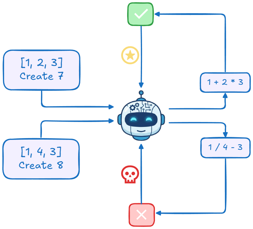
Given a list of numbers (repetitions allowed) and a target value, the goal is to contruct an equation using all (and only) the numbers available in the list to produce target with only +, -, x, / operations.
The exact prompt I used for the model is:
Answer the following question. Provide the reasoning between <reasoning> and </reasoning> symbols. Provide the final answer (an expression) between <answer> and </answer> symbols.\n Using the numbers
[5 96 84 1], create an equation that equals75. You can use basic arithmetic operations (+, -, *, /) and each number can only be used once.
The model was rewarded based on two binary criteria:
- Answer Correctness: The equation produces the target number while abiding by the constraints.
- Format Correctness: Response is formatted in two sections enclosed within the <reasoning> and <answer> XML tags. The Answer Correctness reward is weighted twice compared to Format Correctness.
Base Model
The model being trained is Qwen/Qwen3-4B-Instruct-2507, the largest among the recently released models I could train with my compute availability. This model is also not a ’thinking’ model and so its responses are relatively concise. I believe this also made it easier for the model to learn the context window constraints a little easier. This model scored 71% in answer correctness and 52% in format correctness. This is the score to beat.
Experiments
Initial Setup
I started out with a basic GRPOConfig setting. The effective batch size to 64, with 8 samples per prompt. The completion length was set to 512. All other settings are set to the default values by the trl library as shown below.
Relevant training arguments:
GRPOConfig(
    learning_rate=1e-5,

    gradient_accumulation_steps=64,
    per_device_train_batch_size=8,
    per_device_eval_batch_size=8,

    num_generations=8,

    max_completion_length=512,
    max_prompt_length=256,

    epsilon=0.2,
    epsilon_high=0.2,
    scale_rewards="group",
    reward_weights=[1, 2],
)
I also used LoRA training exclusively with the following configurations:
LoraConfig(
    task_type=TaskType.CAUSAL_LM,
    r=16,
    lora_alpha=32,
    lora_dropout=0.1,
    target_modules=[
        "q_proj", "k_proj", "v_proj",
        "o_proj", "gate_proj", "up_proj", "down_proj"
    ],
)
With these settings, the model learned something but not too well. The test accuracy, without accounting for the formatting issues in the model’s response, improved by about 4%. The model also failed to learn the required output format. And it wasn’t really due to any context length overflow issues that is usually the reason for this. It just forgets to use </reasoning> tag. Here’s an example,
<reasoning>
We are given the numbers: 6, 57, 36, 33
We need to use each number exactly once and combine them using basic arithmetic operations (+, -, *, /) to get a result of 55.

Let’s explore possible combinations.

First, observe that 57 is relatively large. If we subtract
...
57 - 2 = 55 → correct.

This uses all numbers exactly once and only basic operations.

<answer>57 - (6 / (36 - 33))</answer>
Overall, the performance wasn’t really up to expectations.
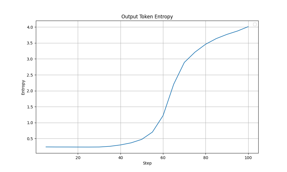
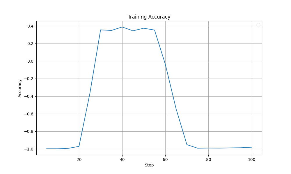
Looking through the training logs, I observed something interesting. The model’s output token entropy exploded around the 50-60 step mark. This coincides with a drop in training accuracy after a plateau that lasted from around step 30. Ideally, the model’s entropy should show a more steady trend since entropy going too high (random tokens) or too low (repetitive tokens) can lead to model collapse.
 |
|---|
| Output Token Entropy during training - Initial Config |
 |
|---|
| Accuracy Reward during training - Initial Config |
Towards A More Stable Training
After the previous result, I made a few changes. I think the major difference is the increased batch size (now 128 x 8) and the increased context length (1024). I also modified some other hyperparams like the epsilon for example.
GRPOConfig(
    learning_rate=1e-5,

    gradient_accumulation_steps=128, # increased 64 -> 128
    per_device_train_batch_size=8,
    per_device_eval_batch_size=8,

    num_generations=8,

    max_completion_length=1024, # increased 512 -> 1024
    max_prompt_length=256,

    epsilon=0.1, # decreased 0.2 -> 0.1
    epsilon_high=0.2,
    scale_rewards=False, # set to False - as suggested by Dr. GRPO paper (https://arxiv.org/pdf/2503.20783)
    reward_weights=[1, 2],
)
The results were quite encouraging. The test accuracy of the model reached 82% (~ 11% improvement over the base model). The format correctness is also 82%. This time the failures were usually the ones on which the model reasoned for too long and ran out of tokens before it could complete the answer. The model seems to have learnt the task and the format quite well.
Here’s a sample answer by the trained model:
Question:
Nums: [5 96 84 1]
Target: 75
Model Response:
<reasoning>
We are given the numbers: 5, 96, 84, and 1. We must use each number exactly once with basic arithmetic operations (+, −, ×, ÷) to form an expression that evaluates to 75.

Let’s first observe that 96 is large and 84 is also large. The target is 75, which is not far from 84. So perhaps we can reduce 84 by something to get to 75.

We can explore:
- 84 - x = 75 → x = 9
- So we need to make 9 from the remaining numbers: 5, 96, and 1.

Alternatively, maybe 96 - something = 75 → something = 21.

Can we make 21 from 5, 84, and 1? 84 is too big. 5×4 = 20, close.

Alternatively, perhaps we can do something like (96 / (something)) to reduce the 96.

Let’s try another angle.

Try combining 96 and 5: 96 / 5 = 19.2 — not promising.

What if we try to use subtraction: 96 - 84 = 12. Then we have 5 and 1 left. Can we make 75 from 12, 5, 1?

12 × 5 = 60, 60 + 1 = 61 — too low.

What if we do (84 - 96) = -12 — not helpful.

Alternatively, try (5 - 1) = 4. Then 96 / 4 = 24. 24 × something?

We have 84 left. 84 / 24 = 3.5 — not helpful.

What if we try to build 75 as a combination of multiplication and addition?

Try: 84 + (5 × 1) = 89 — too big.

Try: 96 - (84 / something)

Try 84 / (96 / x) — not helpful.

Try: 5 × (15) = 75 — so if we can make 15 from 96, 84, and 1?

Can we make 15 from 96, 84, and 1?

(96 - 84) = 12, then 12 + 1 = 13 — not 15.

(84 - 96) = -12 — no.

(96 / (84 / x)) — complicated.

Alternatively, (84 + 96) = 180. 180 / something = 75 → 180 / 75 = 2.4 — not useful.

Wait — 75 = (96 - 84) × 5 + 10? 12 × 5 = 60 + 10 = 70 — close.

Wait — 96 - (84 - (5 × 1)) = 96 - (84 - 5) = 96 - 79 = 17 — not helpful.

Try another idea: can we do (96 × 1) - (84 / something)?

84 / x = 21 → x = 4 — can we make 4 from 5 and 1?

Yes: (5 - 1) = 4.

So: 96 × 1 = 96
84 / (5 - 1) = 84 / 4 = 21
Then 96 - 21 = 75.

Perfect!

We used:
- 96
- 1
- 5
- 84

Each number used once.

Operations: ×, /, −

Expression: 96 - (84 / (5 - 1))

Evaluate:
5 - 1 = 4
84 / 4 = 21
96 - 21 = 75

This works!
</reasoning>

<answer>96 - (84 / (5 - 1))</answer>
Answer Correctness: True
Format Correctness: True
One that the model got wrong:
Question:

Nums: [13 8 60 80]
Target: 44
Model Response:

<reasoning>
We are given the numbers: 13, 8, 60, 80. We need to use each number exactly once and apply basic arithmetic operations (+, −, ×, ÷) to reach the result 44.

Let’s consider possible combinations. The target is 44, which is relatively small compared to 60 and 80. So perhaps we can reduce the larger numbers through subtraction or division.

Try to look for a way to combine 80 and 60 to get something manageable. For example:

80 - 60 = 20. Then we have 13 and 8 left. 20 + 13 = 33, 33 + 8 = 41 — too low.

80 / 60 = 4/3 ≈ 1.33. Not helpful immediately.

What about (80 - 60) = 20. Then 13 * 8 = 104 — too big.

Alternatively, try combining 13 and 8: 13 * 8 = 104. 104 - 80 = 24, 24 + 60 = 84 — too high.

Try (60 / (80 / 8)) = 60 / 10 = 6 — that’s interesting.

So 80 / 8 = 10, 60 / 10 = 6.

Then 13 - 6 = 7 — not helpful.

Alternatively, 80 / (60 / (13 - 8))? Let's test: 13 - 8 = 5, 60 / 5 = 12, 80 / 12 ≈ 6.67 — no.

Try (80 + 13) = 93, 93 - 60 = 33, 33 + 8 = 41 — close.

Try (60 - 8) = 52, 80 - 52 = 28, 28 + 13 = 41 — again close.

What about 80 - (60 / (8 / (13 - 13))) — invalid, division by zero.

Try: (13 * 8) = 104, 104 - 60 = 44 — oh! 104 - 60 = 44.

But we haven’t used 80 yet. So that fails the constraint of using all numbers once.

So we need to use 80 somehow in a way that cancels out or becomes zero.

What if we do: (13 * 8) - 60 + (80 - 80)? But we can’t use 80 twice.

Alternatively, can we use 80 in a division that results in 0 or 1?

Try: (80 - 80) = 0, and 13 * 8 = 104, 104 - 60 = 44. But we used 80 twice.

We can only use each number once.

Another idea: maybe use (80 - 60) = 20, and then (13 - 8) = 5, 20 * 5 = 100 — too big.

(80 - 60) = 20, 20 + 13 = 33, 33 + 8 = 41 — again 41.

(60 - 8) = 52, 52 - 13 = 39, 39 + 80 = 119 — no.

Try combining division: 8 / (13 - 8) = 8 / 5 = 1.6 — not useful.

Try: (60 * 8) = 480, 480 / 80 = 6, then 13 - 6 = 7 — not 44.

(60 + 80) = 140, 140 / something?

140 / x = 44 → x ≈ 3.18 — not matching any of the numbers.

What about: (13 + 8) = 21, 60 / 21 ≈ 2.85 — not helpful.

Another idea: 80 - (60 / (13 - 8)) → 13 - 8 = 5, 60 / 5 = 12, 80 - 12 =
Answer Correctness: False
Format Correctness: False
Reason for failure: Model's reasoning overflowed the context length of 1024 tokens
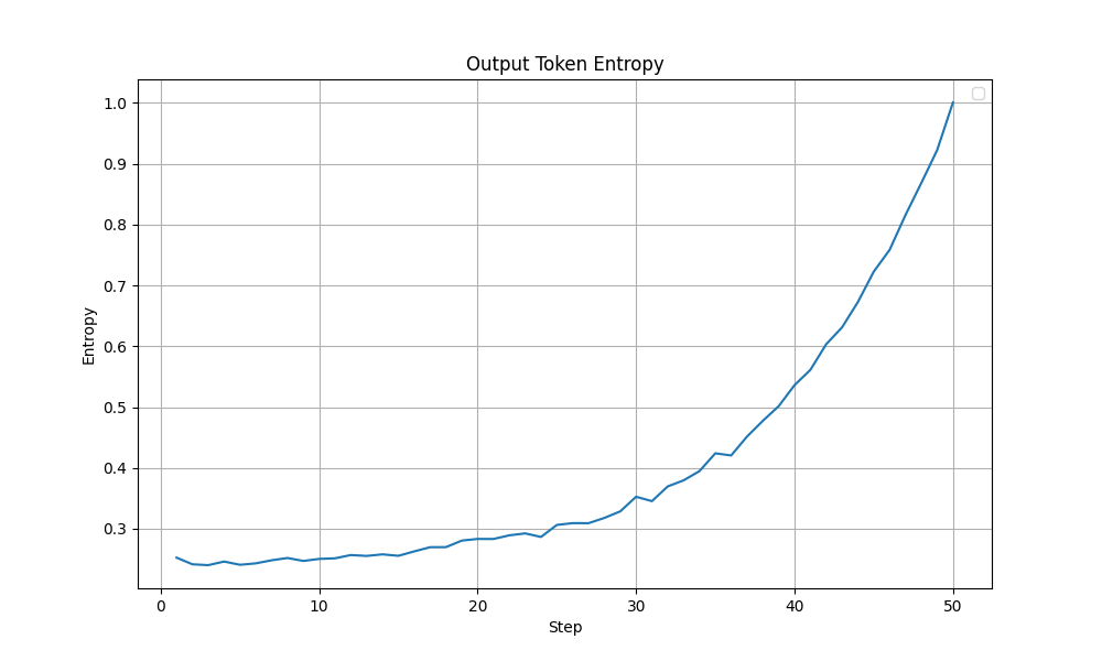
In this experiment, the entropy was better behaved (peaks at ~1.0 with a more steady increase compared to the previous ~4.0). Other metrics like the grad norm and the training loss were also relatively stable. More importantly, the training accuracy improved steadily without any collapse like it was observed before. The graphs are shown below. Overall, I felt this setting was close to optimal and is a good base to start tuning from.
 |
|---|
| Output Token Entropy during training - Improved Config |
 |
|---|
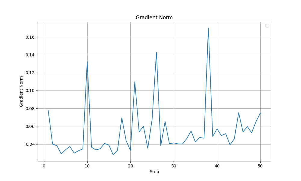
| Grad Norm during training - Improved Config |
 |
|---|
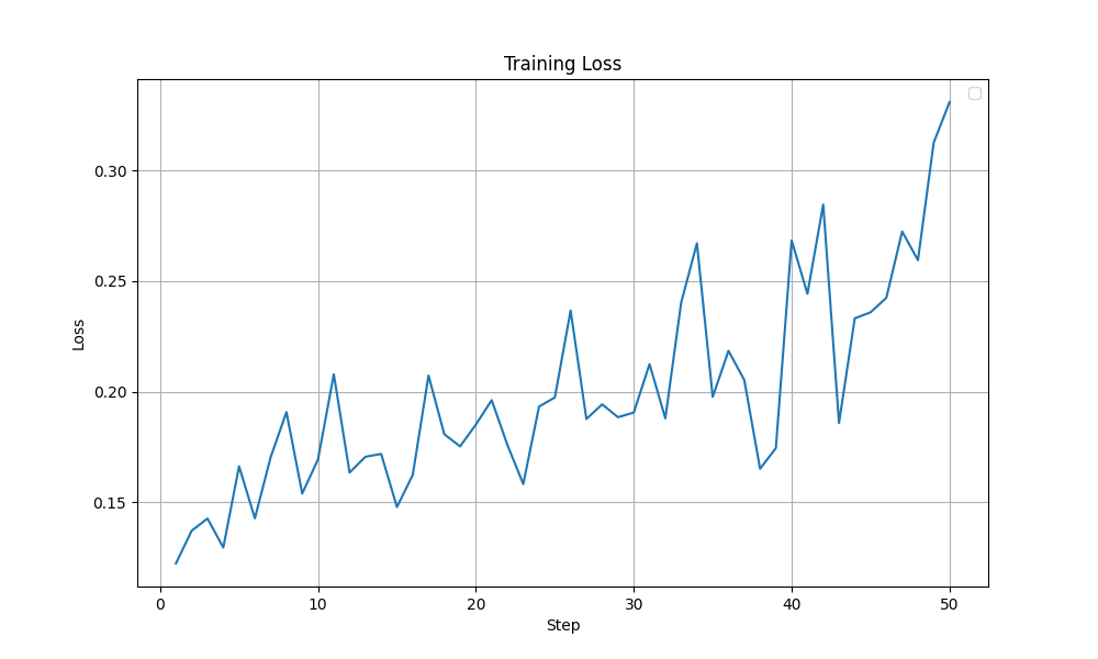
| Loss during training - Improved Config |
 |
|---|
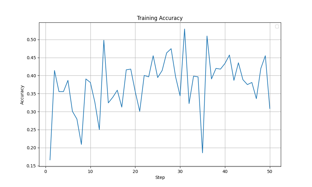
| Accuracy Reward during training - Improved Config |
Pushing It Further
A couple of ideas were considered to improve it further:
- KL divergence - The Grad Norm still showed a lot of spiking suggesting that the gradient updates are not stable enough. Adding a KL divergence penalty might help in controlling the gradient updates. I expected to see changes in the Grad Norm, Entropy and Training Loss curves.
- LoRA linear layers - Midway through my experiments, Thinking Machines dropped this blog on LoRA finetuning. Although all other recommendations were in-line with what I had been using, they find applying LoRA to all linear layers learns better than just applying it to the MLP/Attention layers like I did so far.
KL Divergence
I tested three weight values for KL divergence penalty (beta = $10^{-4}$ vs $10^{-2}$ vs $10^{-1}$). The $10^{-2}$ beta setting worked better and improved from the previous model. There was a 3% improvement in both answer and format correct. Whereas using both $10^{-4}$ and $10^{-1}$ actually ended up performing almost the same as the previous model.
| KL Setting | Answer Correctness | Format Correctness |
|---|---|---|
| 0 | 0.82 | 0.82 |
| $10^{-4}$ | 0.81 | 0.81 |
| $10^{-2}$ | 0.85 | 0.85 |
| $10^{-1}$ | 0.80 | 0.81 |
All Linear Layers For LoRA
I also tried out applying the LoRA adapter for all linear layers with and without a KL divergence penalty. And here surprisingly, the no-KL penalty config outperformed the training run with the KL penalty.
| KL Setting | LoRA layers | Answer Correctness | Format Correctness |
|---|---|---|---|
| 0 | Selected | 0.82 | 0.82 |
| 0 | All-Linear | 0.85 | 0.85 |
| $10^{-2}$ | All-Linear | 0.80 | 0.80 |
I don’t have a strong explanation for what’s happening here but the KL divergence seems to hurt when applying LoRA to all linear layers.
So, Which Is Better?
Although both these modifications, with their best settings achieved the same test accuracy of 85%, looking at the training dynamics, the LoRA training run with selected layers (with beta=1e-2) appears more stable. In the graphs shown below, a sudden drop in Grad Norm, Training Accuracy and Training Loss is observed in the all linear layers run after ~40 steps. The output token entropy also reaches a higher peak (~1.3) than the selected layers run (~0.7). Although it is hard to conclude that that the LoRA training run with selected layers run is more stable, I lean towards the selected layers (with beta=1e-2) configuration.
| Metric | Selected LoRA layers (beta=1e-2) | All Linear (beta=0) |
|---|---|---|
| Train Accuracy | 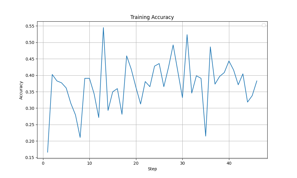 | 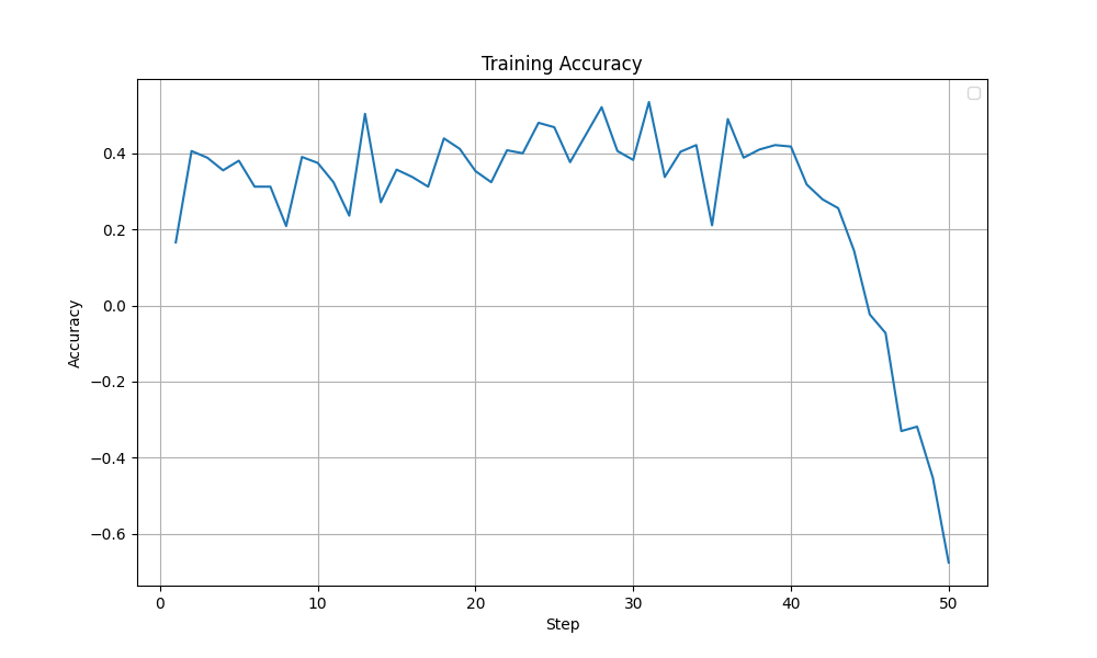 |
| Grad Norm | 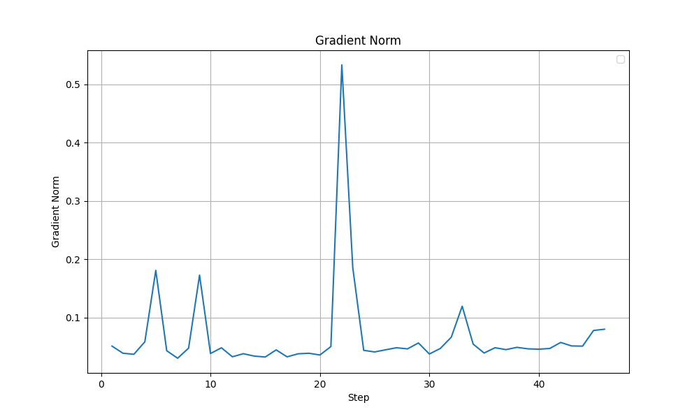 | 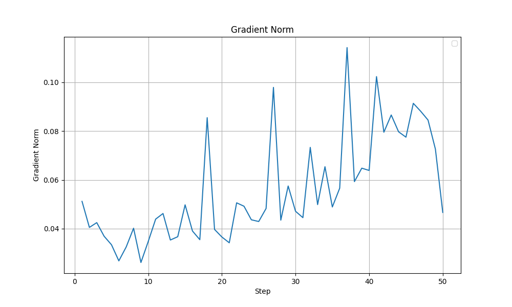 |
| Output Token Entropy | 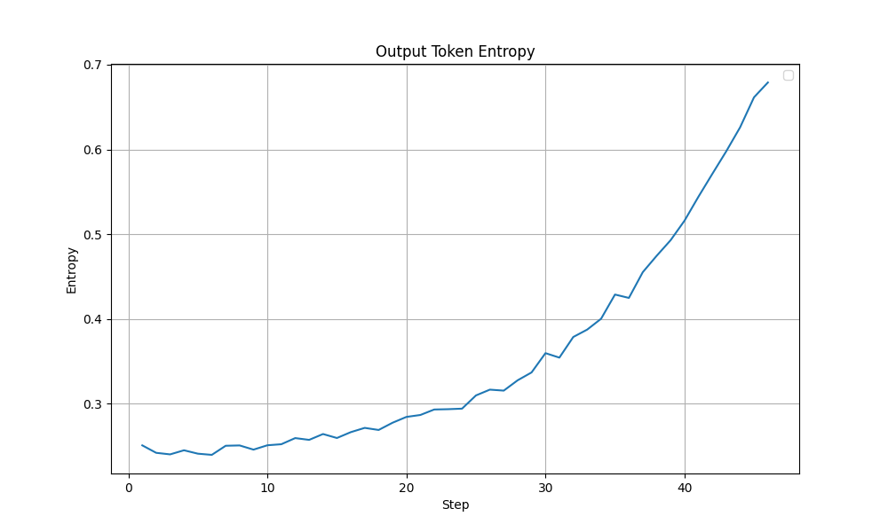 | 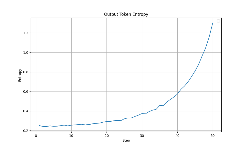 |
| Train Loss | 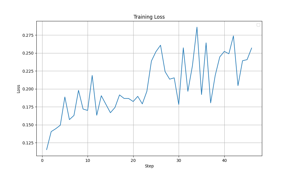 | 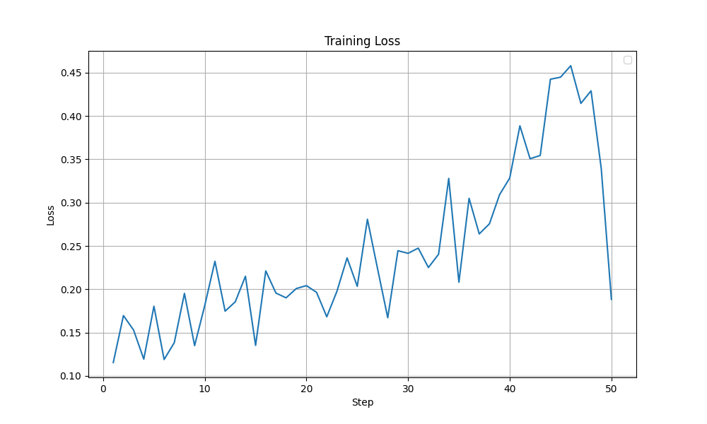 |
Other Experiments
There were also a couple of other side experiments I ran. Their performance wasn’t promising, so I didn’t explore them further.
| Experiment | Description | Answer Correctness | Format Correctness |
|---|---|---|---|
| 0 | N/A | 0.82 | 0.82 |
| Higher Learning Rate | Increased Learning Rate ($10^{-4}$) + KL Divergence Penalty (beta=1e-4) | 0.80 | 0.80 |
| Think tags | Used <think> tag inplace of <reasoning> since I see it being used in the reasoning post-training of the latest thinking models. | 0.79 | 0.79 |
What Am I Working With?
All these experiments were run on a single NVIDIA A40 GPU with 48GB VRAM. The libraries I used were transformers, trl, peft, vllm and tensorboard.
Some Tips To Speed Up Training
- Use
vllmfor generation (use_vllm=True)- It is way faster compared to the
trl’s default generation. - If you only have 1 GPU like myself, use the collocation option (
vllm_mode="colocate") to allowvllmto use the same GPU as theGRPOTrainer. - Use sleep mode (
vllm_enable_sleep_mode=True) to ensure that thevllmmodel is offloaded after the generation so that the VRAM availability for backpropagation (used by theGRPOTrainer) is maximised.
- It is way faster compared to the
- Use LoRA training (I do via
peft)- Training a LoRA adapter is far more memory efficient and faster than full model fine-tuning.
- Another major advantage of LoRA is that it allows you to use the base model (with the LoRA adapter turned off) as the reference model when using KL Divergence penalty. This is huge because you get KL divergence at no extra memory cost while with full finetuning, you need to maintain a whole another copy of the base model.
- Other training settings:
- Gradient Checkpointing (
gradient_checkpointing=True) - Doesn’t store all the intermediate layer outputs during forward pass and so is memory efficient. But recalculating those for backprop will take some extra time. In my case, the tradeoff was worth it. - Mixed Precision Training (
bf16=Trueorfp16=True) - Uses lower precision for most of the computation (like model weights, gradients, activations, etc…) and higher precision for a copy of the model weights for use during the final gradient update step. Results in faster and memory efficient training. - Gradient Accumulation (
gradient_accumulation_steps=n) - Increase the effective batch size by increasing the gradient accumulation steps if you can’t increase theper_device_train_batch_size. In my case, withnum_generations=8andper_device_train_batch_size=8, I was training with exactly 1 prompt in each mini-step. Only with gradient accumulation, I could reach the effective batch size of 128. - Torch Empty Cache (
torch_empty_cache_steps=n) - Frees up cached GPU memory after everynsteps. I setnto1and that gave me some more legroom to work with in the GPU. But this was not as significant as the others.
- Gradient Checkpointing (
Ways to Improve Further
These are things that could improve the performance but I couldnt explore due to hardware limitations.
- Longer context - Because of GPU memory limits, I set the context window to 1024, which I think is enough for this task. But still most task failures is due to context window overflow rather than wrong final equations. So, a longer context will probably help.
- Larger Group Size - I was stuck with
num_generations=8again because of the GPU memory limitations. Maybe setting it to16might produce better results. - Longer training - I ran the training for each configuration for 24 hours, which allowed around 50 steps. Maybe training for longer helps.
Conclusion
With finetuned hyperparameter and training settings, RLVR allowed a 14% improvement in terms of correctness compared to the base model in this toy task. A major factor is probably the increase in effective batch size as it limits the variance in the gradient updates and stabilizes training. Furthermore, adding a KL divergence penalty helped squeeze that final bit of boost in performance. Overall, these experiments gave me a much deeper understanding of the practical intricacies involved in finetuning language models. I hope to try out a more complex task in the future.
Acknowledgements
A huge thank you to Raghavendra Kotikalapudi for guiding me though these experiments and for sharing valuable insights throughout. I learned a lot from our discussions. And thank you to Dr. Mayank Kejriwal for helping me access the compute resources on USC’s CARC without which these experiments would not have been possible.
Resources
Here are some resources that helped me along the way.
- HuggingFace - Ultra-Scale Playbook
- Unsloth - LoRA Hyperparameters Guide
- Thinking Machines - LoRA Without Regret
- nano-aha-moment
Note: An LLM was used in drafting parts of this blog.